PHYCS 3730/6730
Assignment 5 (a05) Optimization, ODEs, PDEs

Exercise 1.

Optimization.

A. In a code deliver.py find as short a path as you can that connects 40 "cities", visiting each city exactly once. The distance between cities is based on 2-d Euclidean geometry and the cartesian coordinate pairs in the file /u/inscc/bromley/courses/ap7730/data/citiesxy.dat (col 1=x, col 2=y, units=km). I recommend NR's Section 10.9 for one approach. Have your code print out the total distance of the path you found, and also submit an x-y line plot of your final path.

Exercise 2.

In this problem we consider the venerable 2-D Ising model, solved by Onsager, to ascertain magnetic properties of a hypothetical 2-D atomic monolayer. In this model, an NxN square lattice (x-y plane with periodic boundaries) has grid points (indices i,j) that represent atoms with spin "up" (S_ij=+1) or "down" (S_ij=-1). Each atom only interacts with its four nearest neighbors: The pairwise interaction energy is E_pair = -J*S_ij*S_i'j' if i,j and i'j' are nearest neighbor sites, while E_pair=0 otherwise. The magnetization of this system is quantified using M=|Sum_ij S_ij|/N^2. In thermal equilibrium, the magnetization depends on temperature T; at low T, all the spins are aligned (M=1); at high T, spins are randomly oriented (M=0). Interesting physics occurs when kT~J.

Write a code, ising2d.py, that estimates M as a function of T using a Monte Carlo method when N=50 and J=0.04 eV. Specifically, have your code take input T (in Kelvin) from the command line, and, starting from some initial state (random spins and M=0 [hot], or identical spins and M=1 [cold]), iterate as follows: Choose a spin, S_ij, and tentatively flip it, calculating the resulting change in energy, dE. If dE is negative (lower energy) accept this new spin, otherwise accept it only with probabiliy exp(-dE/kT). Calculate M as an average value, but only after the system has equilibrate (O(10^6) iterations?). Have your code print out the average (equilibrated) magentization M.

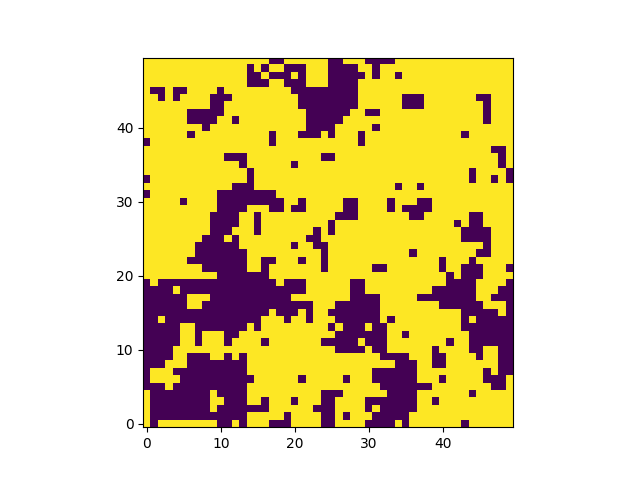
Your MC code will illustrate the physics here: You will find a sharp phase transition at T_crit=2*T_0/ln(1+sqrt(2)), where kT_0=J, distinguishing between M=0 and M=1 regimes. And have fun with this venerable problem! I plotted an image of the output after several million steps, to visualize the growth of spatial correlations in the spin state of the system:
      
 
which shows the pattern of spins (up is yellow, down is purple) for a temperature around T_crit. Other ways to play: What is the impact of "impurities" (e.g., sites with spin S=0)?

Exercise 3.

Integrate the trajectory of the endpoint of a 2-D double pendulum consisting of two rods (with mass m uniformly distributed along each rod of length ell). Choose interesting starting conditions. Choose units where m=1, ell=1, and grav. accel. g=9.8. Plot the trajectory of endpoint of outermost bar for a time t=15. (Caution: this endpoint may be different from the coordinate that is often used in the equations of motion; "(x_i,y_i)" may refer to the center of mass of the i-th bar [i=1,2]). Ensure that energy is conserved to better than one part in 10^4. Change some aspect of your integration (e.g., the choice of output times or suble change in integrator accuracy) to illustrate the sensitivity of the trajectory to numerical effects.

Turn in both your code doublependulum.py and your plot doublependulum.pdf.

Exercise 4.

Solve the 1-D time-dependent Schrodinger equation for a Gaussian pulse impacting a square-well barrier. Use "machine units" (hbar=1,m=1) in a domain of x=[-L/2,L/2] where L=10 units. The starting wave function is

  psi = C*exp(-0.5*((x-x0)/sig)**2)*exp(1j*v0*(x-x0))
  x0 = -2.0; v0 = 50.0; sig=0.125; [C=norm constant; 1j=sqrt(-1)]

Submit your code, schro1d.py, along with a snapshot of |psi|^2 after the final time step, schro1d.png, *or* an animation, schro1d.gif, that spans this final time (and may go beyond it!).