Assignment 2

Exercise 1.

Warm-up: Central limit theorem.

Write a code centrallim.py to illustrate the central limit theorem. With a set of M=[1,2,5,16] independent variates x_i (i=1..M), uniformly distributed over [-1,1], generate N=1000000 samples of x=(x_1+x_2+..x_M)/sqrt(M). Estimate sigma, the std deviation of x, and also the kurtosis k4=(<x^4/sigma^4-3> assuming a zero mean). Have your code print a table, as in

    #  M  sigma  kurtosis  
    #______________________
    #
    1   #####     ######
    2   #####     ######

If it is helpful, formatted printing might be done with

    print('{0:2d} {1:9.6f} {2:9.6f}'.format(m,sig,k4))

where float variables sig and k4 are sdt. dev. and kurtosis, respectively.

Also have your code generate a plot, centrallim.pdf, showing superimposed histograms for all four values of M. If you use matplotlib's hist() function, please use histtype='step' and density=True for easy comparison.

[The takeaway is the convergence of non-Gaussian processes converge "normality" as predicted by the Central Limit Theorem. I played around with various other starting distributions like x=u^3 and (of course) x=random.normal() to get a sense of the effect of finite sample size....]

Exercise 2.

The hypervelocity star LAMOST-HVS1 (discovered by Prof. Zheng and collaborators! see Zheng et al. 2014) is moving so fast that it will escape from our Galaxy. The Gaia astrometry mission also observed this star (designated as Gaia DR2 590511484409775360). From the Gaia observations, this star moves across the sky at an angular velocity of

  mu_x = -3.537 +/- 0.110 (mas/year [RA dir], 1-sigma error)
  mu_y = -0.620 +/- 0.093 (mas/year [dec dir])
  rho = -0.2516 (correlation coefficient of mu_x and mu_y)

The units are milli-arcseconds (mas) per year, where 1 mas=4.8481368e-9 radians; "x" and "y" refer to horizontal and vertical directions of travel across a tiny patch of sky. (Details for astronomers: x is along right ascension and y is declination). The uncertainties listed are "1-sigma errors" (68% confidence range) and the error distributions of these measurements are well-approximated as Gaussian.

In a python script called lamost_hvs1.py, use Monte Carlo trials to estimate the angular speed, mu, in (mas/year), reporting the median speed with upper and lower error bounds that define a 68% confidence region (lower bound, upper bound are 16th-percentile and 84th-percentile of the possible mu values). Note: in astronomy this angular movement is known as "proper motion".

Hint: if you choose to use the emcee package (see info at this informal link and specifically this link with info for this problem) you might be able to easily adopt your code to the next exercise.

Exercise 3.

Another star, Gaia DR2 1540013339194597376, was recently identified (see Table 3 of this article) as being a potential hypervelocity star (unbound to the Galaxy, like LAMOST-HVS1). The distance to this star from us is estimated using its parallax, the change in the star's position in the sky from the Earth's orbit around the Sun. This star's parallax is

pax = 0.5894 +/- 0.0528 mas

where the uncertainty is sigma, the std dev of a Gaussian error distribution. If parallax were known perfectly, it would give the star's distance from the Sun as dist=1/pax, in units of kiloparsecs (kpc, 3.08e19 m) when pax is in mas (see previous exercise). The angular drift speed of this star (a.k.a., its proper motion) is mu=143.9 mas/year with errors below0.1 mas/year, which you may ignore here.

In a MCMC code called faststar.py, find the speed v_sky=mu*dist of this star in the plane of the sky, perpendicular to the line of sight between the star and the Sun. Report your result, and 68.3% confidence limits (16th and 84th percentiles), in units of km/s. Do this calculation in two ways:

Assume that the distance is drawn from error distribution
p(dist|pax)~exp(-(pax-1/dist)^2/(2*sigma^2))*|dpax/ddist|
where pax is the measured distance and |dpax/ddist| is a Jacobian. This is a minimalist approach in that we assert only the conservation of probability in a change of variables [p(y)dy=p(x)dx]. [Note: The Jacobian is not needed if the mcmc sample variable is itself z=1/pax, and if the samples are converted to distance d=1/z].
Use a Bayesian prior, a distance distribution of that expresses our assumptions on the true distance of the star. [Formally, we want to estimate the posterior distribution, p(y|x)~p(x|y)p(y), where p(y) is the prior]. Draw MCMC distance samples from
p(dist|pax)~exp(-(pax-1/dist)^2/(2*sigma^2))*[dist^2*exp(-dist/lambda)]
The term in the "[]" is the prior, and it reflects an expectation that stars in the Gaia survey most likely lie close to the Sun. Set lambda=0.1 kpc, meaning that we expect most stars to be within a kpc of the Sun.

In addition to the two speed estimates, have your code generate histograms of the predicted speed distribution of the star in file faststar.pdf.

Hints/comments:

Conversion: 1 (mas/year)*kpc = 4.740505 km/s.
The reference frame for this problem is the Sun's rest frame. The full problem of identifying a hypervelocity star requires changing to the Galaxy's rest frame. Still, since the Sun's speed in the Galaxy is known, 240 km/s, we say something about whether the star discussed here is bound to the Galaxy or not.
I estimate a speed that is much higher than the local escape speed of the Galaxy (about 600 km/s). The idea in using the prior is to force a more realistic the distance estimate that happens to reduce the star's speed.
The choice of prior parameter lambda=0.1 kpc is unrealistically small (see for example).

Exercise 4.

The time series in files

~bromley/courses/ap7730/data/GW150914_H.dat
~bromley/courses/ap7730/data/GW150914_L.dat

have the strain signal from the first binary black hole merger event, GW150914, reported by LIGO. The first file is from the Hanford (WA) and Livingston (LA) detectors. These are text files with a single column of data, samples of the strain taken at a rate of 4096 HZ, spanning 32 seconds, and starting at a time specified in the file in a common time coordinate system. These files were downloaded from. this link

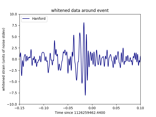
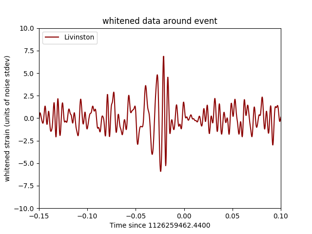
The processing that the LIGO team uses to extract the signal is elegant. But the signal can at least be verified using a simple procedure involving a passband filter based on the power spectral density of the two data streams. The exercise here is to build this simple filter to extract the strain signal in the two time series.

Write a script, gravwave.py, that does the filtering and generates a plot, gravwave.pdf, showing the strain in a 0.3 second time interval bracketing the event for both the Hanford and Livingston data (on trhe same plot). In the time coordinates correspondng to the data in the files, the time of the event is t=1126259462.44 seconds. In your plot, show time such that the event is at t=0 on the horizontal axis, and the signal strength in the vertical axis is in units of noise std dev (referring to the standard deviation of the filtered strain samples). These images show the LIGO team's results

Here, you are after something similiar, not in exact wave form but in signal strength.

Details and hints.

Process each of the two time series separately. Just a heads up, the GW signal is located almost midway in the time teries and lasts roughly 0.1 sec. The Hanford and Livingston data streams are offset by 1 second (one begins t=1 s before the other; see the fiorst two lines of each file).
Have your code expect the data to be either in the working directory or use the absolute path to the files. One option for reading the files is numpy's loadtxt().
Scipy's signal.welsh() provides an estimate of the PSD. It returns two arrays (the frequencies and the PSD evaluated at those frequencits). The frequencies will have physical values [units of Hz] if you call welsh() with arg fs=4096, which is the sampling rate of the data,
Use scipy's interp1d() to create a function based on welsh()'s returned arrays so that you can get interpolated values of the PSD at arbitrary frequencies.
Numpy's fft.rfft takes the fast Fourier transform (FFT) of a real function, returning it as an array. Calling np.fft.rfftfreq(nt,dt) [where dt=1./4096.0 and nt is the number of points in the time series] gets an array with the corresponding frequencies.
Create a filter W as an array constaining 1/np.sqrt(PSD), being sure to evaluate W at all the frequencies involved in the FFT [this is why interp1d() is needed]. Also mask out frequencies below a certain value [TBD; I tried 20-50 Hz] and above about 300 Hz. Using 1/sqrt(PSD) "whitens" data (makes the power more evenly distributed across the frequency spectrum like white light) by upweighting weak signal and downweighting strong signals at specific frequencies. Clipping both low and hi frequencies selects part of the spectrum where the LIGO observatories are sensitive to astrophysical signals.
Do an inverse FFT (irfft) to get back into the time domain.
Estimate the background noise level by calculating the std dev of the filtered time series (it's mostly noise, even when GWs are detected!). NB: after filtering, the time series may have "edge" artifacts at the beginning and end points, so I would mask out/remove the first and last 5 seconds of the time series.

Once you have your code working, there are lots of cool things to try. Examples include cross-correlating the two signals to figure out the lag, fitting wave forms, trying to pluck out the sinusoidal-ish signal before the chirp... In creating this problem, I worked from this website, very cool, shows the right way of approaching the data management and signal processing....Enjoy!

Submit your answers.

submit p7730 a02 .....