source: NASA
For each of the following exercises create a text file with your answer. See Exercise 3, below, for instructions for submitting your homework.
The probability of finding a ground-state electron at radial distance [r,r+dr] from the nucleus of a hydrogen atom is
p(r) = C*r^2*exp(-2*r) (0<r<10)where C is a normalization constant and r is in units of Bohr radii (5.26e-9 cm). In a python script called electrondist.py do the following:
a) Calculate the mean distance <r> and the second moment <r> Find P(r<1), the probability that the electron lies inside of r=1. Specifically, do so first with hand-coded Simpson's rule with n=11 points, then with scipy's Gaussian quadrature routing, keeping the relative error below 1e-8. [See part (c) for how to report your results.]
b) Generate N=10^5 samples of a random variate that is distributed as in the above equation. Specifically, calculate the cumulative distribution function P(r<R) on a grid of uniformly spaced values of R=0..10. Invert this function to get R = CDF^-1, such that if you pick a value u, so that u=CDF, you can get R=CFD^-1(u). (A linear interpolator might be useful here, cubic spline seems dangerous?) Then, choose N values of u, randomly and uniformly distributed between 0 and 1, converting them into samples of radial distance r. Create a histogram of the N samples in part (b) in a file called electrondist.pdf, and use these samples to estimate the mean of r and the second moment, reporting your results as described next.
c) Have your code print out your results from parts (a) and (b) as follows:
mean(For the analytical estimate, maple or mathematica might help.)
Simpson n=11: #####
Quadrature: ##### +/- #####
Random trials: Analytical: #####
second moment
Simpson n=11: #####
Quadrature: ##### +/- #####
Random trials:
Analytical: #####
Write a python script, sphere12d.py, to estimate the volume of a unit sphere in 12-D using Monte Carlo integration. Estimate the error (std deviation of the mean value of the integral) and stop the integration when the fractional error falls below 1%.
Have your code print out your result in this format:
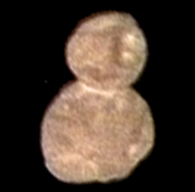
NASA's New Horizons mission recently flew past Ultima Thule (2014 MU_69), a "contact binary" Kuiper belt object, capturing this image:
source: NASA
Assume that this object can be described as two spheres with radii r_u=9.5 km and r_t=7.0 km, with centers separated by a distance d = 14.5 km. The subscripts u and t are for "Ultima" (the name of the larger binary partner) amd "Thule" (the smaller partner). Note that the spheres formally overlap; for the purpose of this exercise, suppose Ultima is exactly spherical, while Thule is spherical except for the part that extends into Ultima. Assume also that the mass density of the binary is a constant, ρ=0.8 g/cm^3.
Define a rectilinear coordinate system wherein the centers of Ultima and Thule lie on the x axis, with Ultima located at some negative value, x_u<0, and with the center of mass of the system is at the origin. Find
(a) x_u and x_t, corresponding to the location on the x axis of Ultima and Thule, repsectively (in km);
(b) U_rotate, the rotational energy of the system (in ergs), assuming solid body rotation about the z axis with a period T=15 hours; and
(c) U_grav (in ergs), the gravitational binding energy of the binary, i.e., the energy reguired to separate Thule from Ultima (in ergs).
Turn in a single python script, ultima-thule.py that does these calculations numerically and prints results clearly, as in:
x_u = ##### kmBe sure that your answers are accurate to within 0.1%. In this case, the simple geometry of the problem allows for easy analytical estimates as a check.
x_t = ##### km
[How did the contact binary form? the rotational energy versus the gravitational binding energy is one clue.]
Please follow the instructions given here in the assignments web page.
Files to turn in: